Udacity A/B Testing Project
Table of Contents Link to heading
- 0. Experiment Description
- 1. Experiment Design
- 2. Metric Choices
- 3. Measure of Variability
- 4. Sizing
- 5. Sanity Check
- 6. Effect Size Tests
- 7. Sign Test
- 8. Recommendation
0. Experiment Description Link to heading
Currently, the Udacity course home pages offer two options: “start free trial” and “access course materials.” By selecting “start free trial,” users are prompted to enter credit card information and are then enrolled in a 14-day trial period, followed by automatic charges. Alternatively, choosing “access course materials” allows users to view the course content but excludes coaching support, verified certificates, and project feedback.
The rationale behind this change is to allocate study time for students, potentially enhancing the overall student experience and enabling coaches to better support students who are likely to complete the course. The goal of the experiment is reducing the number of students who would quit the course during the starting 14days period, while leaving the number of studnets who pass this 14days period intact. I would like to call the first group of students, “frustrated”, and the second group, “resolute” students.
1. Experiment Design Link to heading
The initial unit of diversion to the control and experiment groups is a unique cookie. However, once a student enrolls in the free trial, they are tracked by user-id. The same user-id can’t enroll more than once. Users who don’t enroll are not tracked by user-id. The uniqueness of a cookie is determined per day.
2. Metric Choices Link to heading
We need two groups of metrics. One group for measuring the effect of change that is imposed, and one group for sanity check, i.e. validation of the test.
2.1. Invariant Metrics Link to heading
2.1.1. Number of cookies: The number of unique cookies to visit the course overview page. This is the unit of diversion and even distribution amongst the control and experiment groups is expected. It is therefore appropriate as an invariant metric.
2.1.2. Number of clicks: The number of users (tracked as unique cookies at this stage) to click the free trial button. This is appropriate as an invariant metric but not an evaluation metrics. Equal distribution amongst the experiment and control groups would be expected since at this point in the funnel the experience is the same for all users and therefore elements of the experiment would not be expected to impact clicking the “start free trial” button.
2.1.3. Click-through-probability: Unique cookies to click the “start free trial” button per unique cookies to view the course overview page. Equal distribution amongst the experiment and control groups would be expected since at this point in the funnel the experience is the same for all users and therefore elements of the experiment would not be expected to impact clicking the “start free trial” button.
2.2. Evaluation Metrics Link to heading
Evaluation metrics were chosen since there is the possibility of different distributions between experiment and control groups as a function of the experiment. Each evaluation metric is associated with a minimum difference (dmin) that must be observed for consideration in the decision to launch the experiment. The ultimate goal is to minimize student frustration and satisfaction and to most effectively use limited coaching resources. Cancelling early may be one indication of frustration or low satisfaction and the more students enrolled in the course who do not make at least one payment, much less finish the course, the less coaching resources are being used effectively. With this in mind, in order to consider launching the experiment either of the following must be observed:
2.2.1. Gross conversion: That is, number of user-ids to complete checkout and enroll in the free trial divided by number of unique cookies to click the “Start free trial” button. (dmin= 0.01) - It can be an evaluation metric. The value should be reduced in the experiment group since the number of enrollments is expected to decrease.
2.2.2. Retention: That is, number of user-ids to remain enrolled past the 14-day boundary (and thus make at least one payment) divided by number of user-ids to complete checkout. (dmin=0.01) - This can be an evaluation metric. Since we expect that the number of enrollment reduces, and the number of payments remains more or less the same, this metric is expected to be more in the experiment group comparing to the control group.
2.2.3. Net conversion: That is, number of user-ids to remain enrolled past the 14-day boundary (and thus make at least one payment) divided by the number of unique cookies to click the “Start free trial” button. (dmin= 0.0075) - This can be an evaluation metric. The number of clicks is unaffected by the change, the number of payments is expected to remain more or less the same, so the change of this metric is expected to be insignificant.
3. Measure of Variability Link to heading
It is asked in the template to calculate the “standard deviation of the sampling distribution” or standard error(SE). The standard error of the current metrics depends on the sample size, and can be computed analytically.
Since the daily unique cookies of the overview page is 5000, we need to figure out sample size for each metric. The sample size is equal to the denominator quantity, assuming 5000 unique cookies for the overview page.
The formula which is used here for estimation of the standard error is based on CLT, and the fact that sampling distribution of the metrics has normal distribution.
p_enroll_click <- 0.20625
n <- 400
SE_gross_conversion <- sqrt(p_enroll_click*(1-p_enroll_click)/n)
SE_gross_conversion
## [1] 0.0202306
p_payment_enroll <- 0.53
n <- 82.5
SE_retention <- sqrt(p_payment_enroll*(1-p_payment_enroll)/n)
SE_retention
## [1] 0.05494901
p_payment_click <- 0.1093125
n <- 400
SE_net_conversion <- sqrt(p_payment_click*(1-p_payment_click)/n)
SE_net_conversion
## [1] 0.01560154
4. Sizing Link to heading
| Unique cookies to view page per day: | 40000 |
|---|---|
| Unique cookies to click “Start free trial” per day: | 3200 |
| Enrollments per day: | 660 |
| Click-through-probability on “Start free trial”: | 0.08 |
| Probability of enrolling, given click: | 0.20625 |
5. Sanity Check Link to heading
The first step in validation of the experiment is assessment of invariant metrics. There are some metrics that are expected to have more or less identical values in the both experiment and control groups.
From the metrics that we have, I have chosen the number of cookies, number of clicks, and click-through probability as invariant metrics. Now using this data, I check whether the values of these metrics are significantly different in the experiment and control groups.
control <- read.csv("/Users/yuxishen/Downloads/Final\ Project\ Results\ -\ Control.csv")

experiment <- read.csv("/Users/yuxishen/Downloads/Final\ Project\ Results\ -\ Experiment.csv")
For the counts metrics, we assumed that 50% of the experiment traffic goes to the experiment group and 50% goes to the control group. If we call these two groups success and failure, then the model can be a Bernoulli distribution. So I would check whether the current counts of these two groups can come from a population with 0.5 change of success or failure. And I do it using bootstrapping to estimate and build confidence interval.
Null Hypothesis: Status quo. Any difference between the metric value of the two groups is due to chance. Alternate Hypothesis: The difference between the metric value of the two groups is meaningful, and significant. It cannot be due to random change.
It is said in the course that we should calculate the fraction of the control group on the total. It can be the difference of the numbers of the two groups, or relative size of each group to another one. There are different ways anyway.
The calculation:
alpha <- 0.05

experiment_pageviews <- experiment$Pageviews
total_exp_pview <- sum(experiment_pageviews)
total_exp_pview
## [1] 344660
control_pageviews <- control$Pageviews
total_cntl_pview <- sum(control_pageviews)
total_cntl_pview
## [1] 345543
observed_ratio<- total_cntl_pview/
        (total_exp_pview+total_cntl_pview)
observed_ratio
## [1] 0.5006397
pool <- c(rep(x= 1,total_cntl_pview),rep(0,total_exp_pview))
ratio_vector <- vector(length=10000)

#sum(pool)/length(pool)

# Calculation Using for-loop
#----------------------------
# for (i in 1:10000){
#         pool_resample <- sample(pool,
#                                 size = length(pool),
#                                 replace = TRUE)
#
#         ratio_vector[i] <- sum(pool_resample)/length(pool)
# }
#
# hist(ratio_vector)
# abline(v = observed_ratio)
# --------------------------
# Calculation Using lapply()
#----------------------------
# t<- lapply(1:10000 , function(i){
#         pool_resample <- sample(pool,
#                                 size = length(pool),
#                                 replace = TRUE)
#
#         ratio_vector[i] <- sum(pool_resample)/length(pool)
#         #ratio_vector[i]
# })
#
# t <- unlist(t)
# hist(t)
# -----------------------------
#Calculation using parallel computing
#----------------------------

# Calculate the number of cores
no_cores <- detectCores() - 1

# Initiate cluster
cl <- makeCluster(no_cores)


t_parallel<- mclapply(X = 1:10000 , FUN = function(i){
        pool_resample <- sample(pool,
                                size = length(pool),
                                replace = TRUE)

        ratio_vector[i] <- sum(pool_resample)/length(pool)
        #ratio_vector[i]
} )

t_parallel <- unlist(t_parallel)
t_parallel <- sort(t_parallel,decreasing = FALSE)
lower_bound <- t_parallel[10000*alpha/2]
upper_bound <- t_parallel[10000 - (10000*alpha/2)]

hist(t_parallel, main = "Proportion of #cookies" )
abline(v =0.5 , col = "blue" )
abline(v = lower_bound, col = "red")
abline(v = upper_bound, col = "red")
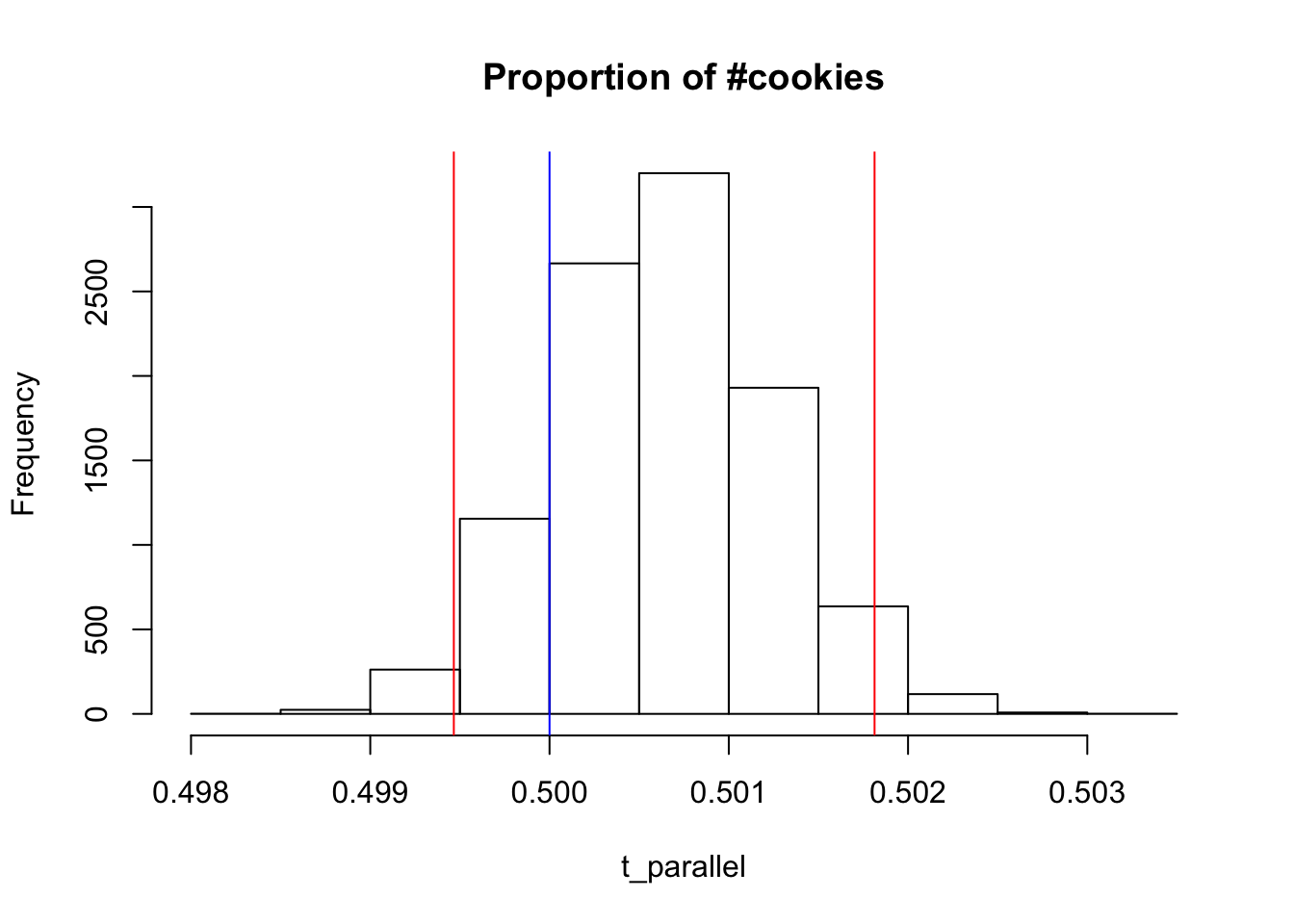
Again it is clear that the number of clicks is randomly assigned into the experiment and control groups.
The last sanity check would be evaluation of the click-through-probability. Bootstrapping would help in this case too. What we want to measure is the significance of the difference between the click-through probability of the experiment and control groups.
One approach is calculation of the difference vector, then building confidence interval around its average using resampling method.
experiment_ctp <- experiment$Clicks / experiment$Pageviews
control_ctp <- control$Clicks / control$Pageviews

diff_ctp <- round(experiment_ctp,4) - round(control_ctp,4)
obs_diff_avg <- mean(diff_ctp)
obs_diff_avg
## [1] 6.486486e-05
Now the bootstrapping.
diff_avg_vector <- vector(length=10000)


ctp_parallel<- mclapply(X = 1:10000 , FUN = function(i){
        pool_resample <- sample(diff_ctp,
                                size = length(diff_ctp),
                                replace = TRUE)

        diff_avg_vector[i] <- mean(pool_resample)

} )

ctp_parallel <- unlist(ctp_parallel)
ctp_parallel <- sort(ctp_parallel,decreasing = FALSE)
lower_bound <- ctp_parallel[10000*alpha/2]
upper_bound <- ctp_parallel[10000 - (10000*alpha/2)]

hist(ctp_parallel, xlab = "CTP diff between two groups")
abline(v =0 , col = "blue" )
abline(v = lower_bound, col = "red")
abline(v = upper_bound, col = "red")
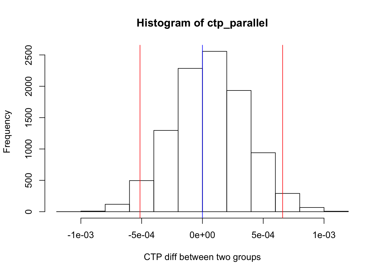
As it can be seen, 0 is in the CI so the difference between the two groups is insignificant.
6. Effect Size Tests Link to heading
As all sanity checks were passed, and the experiment data is validated to some extent, we can go forward and analyze the evaluation metrics.
What we want to do is assessing whether the differences between evaluation metric values of the control and experiment groups are significant or not. Previously, we had chosen gross conversion and net conversion as the two evaluation metrics. We expect the gross conversion to be lower in the experiment group since the number of enrollments should be lowered, and in contrast we expect not to see any significant difference between the values of net conversion rate of the experiment and control groups.
experiment_net_c <- experiment$Payments/experiment$Clicks
experiment_net_c <- experiment_net_c[!is.na(experiment_net_c)]

control_net_c <- control$Payments/control$Clicks
control_net_c <- control_net_c[!is.na(control_net_c)]

diff_net_c <- experiment_net_c - control_net_c
avg_net_c <- mean(diff_net_c)
avg_net_c
## [1] -0.004896857
It is interesting that the net conversion value is negative, so the net conversion rate in the experiment group is lower than the control group.
Now we can use bootstrapping to check whether the observed value is exceptional under given alpha and assumed null hypothesis.
net_c_avg_vector <- vector(length=10000)

pool <- c(experiment_net_c, control_net_c)

net_c_parallel<- mclapply(X = 1:10000 , FUN = function(i){

        # exp_resample <- sample(pool,
        #                         size = length(experiment_net_c),
        #                         replace = TRUE)
        # cntl_resample <- sample(pool,
        #                         size = length(experiment_net_c),
        #                         replace = TRUE)
        # net_c_avg_vector[i] <- mean(exp_resample - cntl_resample)


        resample <- sample(diff_net_c,
                           size = length(diff_net_c),
                           replace = TRUE)
        net_c_avg_vector[i] <- mean(resample)


} )

net_c_parallel <- unlist(net_c_parallel)
net_c_parallel <- sort(net_c_parallel,decreasing = FALSE)
lower_bound <- net_c_parallel[10000*alpha/2]
upper_bound <- net_c_parallel[10000 - (10000*alpha/2)]

hist(net_c_parallel, xlab = "Net C diff between two groups")
abline(v =0 , col = "blue" )
abline(v = lower_bound, col = "red")
abline(v = upper_bound, col = "red")
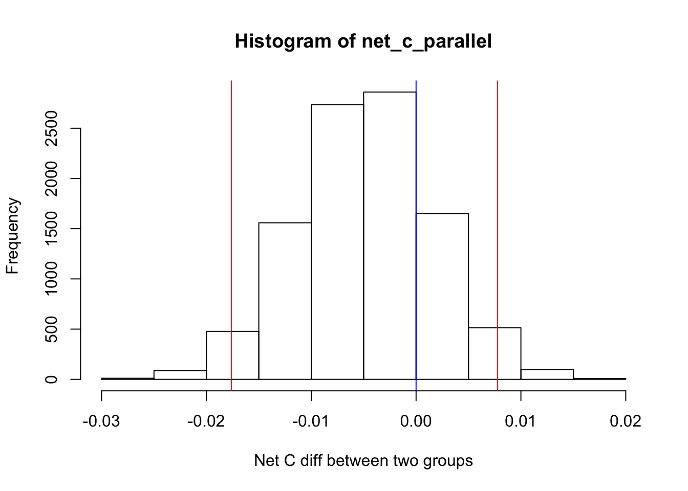
As it can be seen, the difference between net conversion rate of the two expriment and control groups is insignificant. This is exactly what we expected.
The second metric is the gross conversion rate. The analysis would be exactly the same as above, but we expect a significant result for this metric. More specifically, it is expected that this metric is significantly lower in the experiment group comparing to the control group.
experiment_gross_c <- experiment$Enrollments/experiment$Clicks
experiment_gross_c <- experiment_gross_c[!is.na(experiment_gross_c)]

control_gross_c <- control$Enrollments/control$Clicks
control_gross_c <- control_gross_c[!is.na(control_gross_c)]

diff_gross_c <- experiment_gross_c - control_gross_c
avg_gross_c <- mean(diff_gross_c)
avg_gross_c
## [1] -0.02078458
The observed difference is negative, showing that the metric in the experiment group is lower than the metric in the control group.
Now bootstrapping based on the null hypothesis.
gross_c_avg_vector <- vector(length = 10000)

gross_c_parallel<- mclapply(X = 1:10000 , FUN = function(i){

        resample <- sample(diff_gross_c,
                                size = length(diff_gross_c),
                                replace = TRUE)


        gross_c_avg_vector[i] <- mean(resample)

} )

gross_c_parallel <- unlist(gross_c_parallel)
gross_c_parallel <- sort(gross_c_parallel,decreasing = FALSE)
lower_bound <- gross_c_parallel[10000*alpha/2]
upper_bound <- gross_c_parallel[10000 - (10000*alpha/2)]

hist(gross_c_parallel, xlab = "CI of the observerd Gross Conv Rates")
abline(v =0 , col = "blue" )
abline(v = lower_bound, col = "red")
abline(v = upper_bound, col = "red")
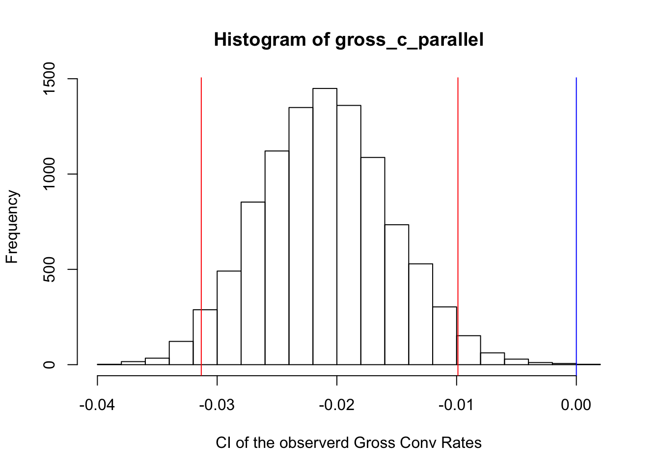
As it can be seen, the 0 is out of CI boundary, and it shows that the obsevered result is statistically significant. Also since the result is on the left hand side of the 0, our expectation is met and the gross conversion rate of the experiment group is lower than the control group.
7. Sign Test Link to heading
Sign test is basically checking whether the signs, either positive or negative, of the differences of the metrics between two groups are meaningfully distributed over the days of the experiment or not. For instance, if in every single day of the experiment the gross conversion rate is lower in the experiment group comparing to the control group, then being so assures us further that this metric is significantly reduced due to the experiment.
In order to check the significance of the signs, it is possible to use bootstrapping as well. The null hypothesis is the proportion of negative signs to the number of experiment days is a random and insignificant value. Thus, this is a one sample proportion test.
For the net conversion rate sign test, I consider being negative as the baseline, and I check whether the observed number of negative values is statsitically significant or not.
net_c_sign <- diff_net_c < 0

#the observed proportion of negative signs
net_c_prop<- sum(net_c_sign)/length(net_c_sign)
net_c_prop
## [1] 0.5652174
net_c_sign_vector <- vector(length = 10000)
net_c_sign_parallel<- mclapply(X = 1:10000 , FUN = function(i){

        resample <- sample(net_c_sign,
                                size = length(net_c_sign),
                                replace = TRUE)


        net_c_sign_vector[i] <- sum(resample)/length(resample)

} )

net_c_sign_parallel <- unlist(net_c_sign_parallel)
net_c_sign_parallel <- sort(net_c_sign_parallel,decreasing = FALSE)
lower_bound <- net_c_sign_parallel[10000*alpha/2]
upper_bound <- net_c_sign_parallel[10000 - (10000*alpha/2)]

hist(x = net_c_sign_parallel, xlab = "Net conversion sign CI")
abline(v =0.5 , col = "blue" )
abline(v = lower_bound, col = "red")
abline(v = upper_bound, col = "red")
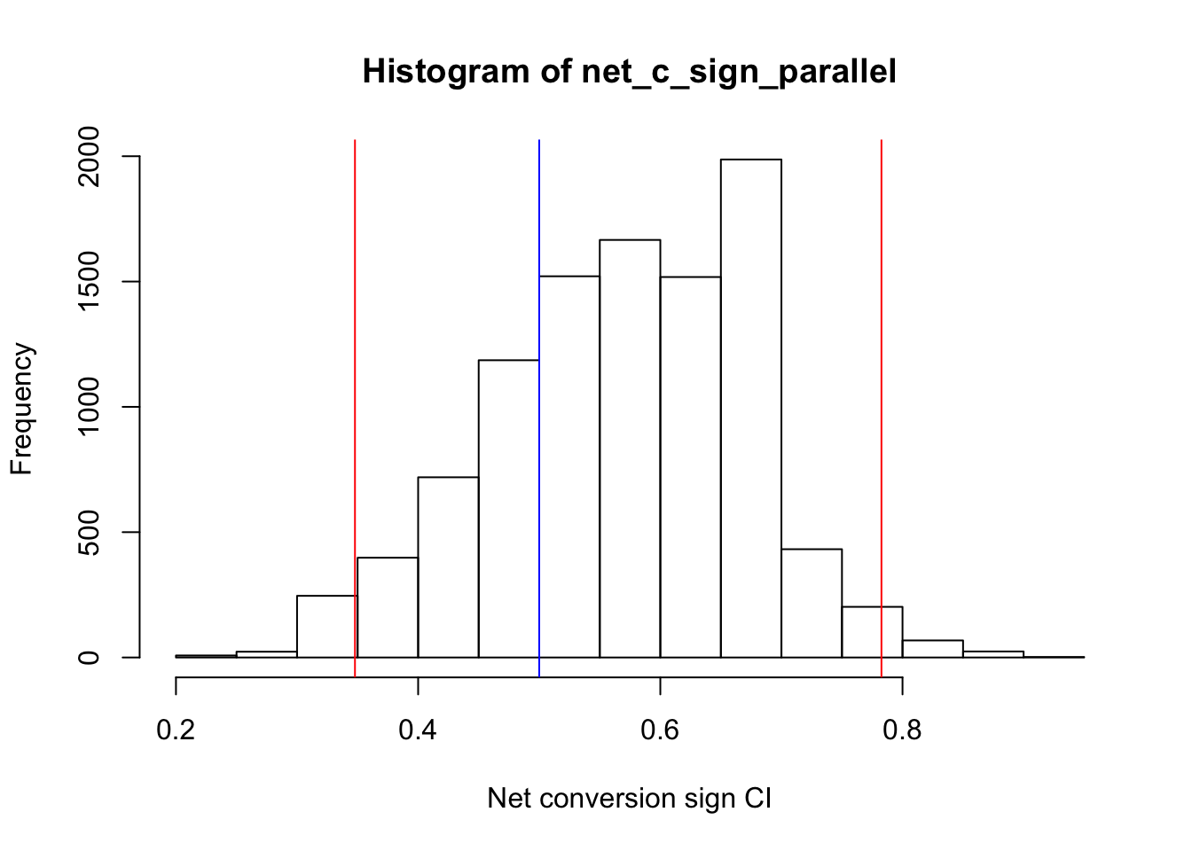
So the above graph shows that the observed sign data for the net conversion is totally regular, and there is nothing exeptional based on the significance level of alpha. The CI of the observed data includes 0.5 proportion, so there is no reason not to believe that this data comes from a population with proportion value = 0.5.
We do the same for the gross conversion rate.
gross_c_sign <- diff_gross_c < 0

#the observed number of negative signs
gross_c_prop <- sum(gross_c_sign)/length(gross_c_sign)
gross_c_prop
## [1] 0.826087
gross_c_sign_vector <- vector(length = 10000)
gross_c_sign_parallel<- mclapply(X = 1:10000 , FUN = function(i){

        resample <- sample(gross_c_sign,
                                size = length(gross_c_sign),
                                replace = TRUE)


        gross_c_sign_vector[i] <- sum(resample)/length(resample)

} )

gross_c_sign_parallel <- unlist(gross_c_sign_parallel)
gross_c_sign_parallel <- sort(gross_c_sign_parallel,
                              decreasing = FALSE)
lower_bound <- gross_c_sign_parallel[10000*alpha/2]
upper_bound <- gross_c_sign_parallel[10000 - (10000*alpha/2)]

hist(gross_c_sign_parallel, xlab = "Gross conversion sign CI")
abline(v =0.5 , col = "blue" )
abline(v = lower_bound, col = "red")
abline(v = upper_bound, col = "red")
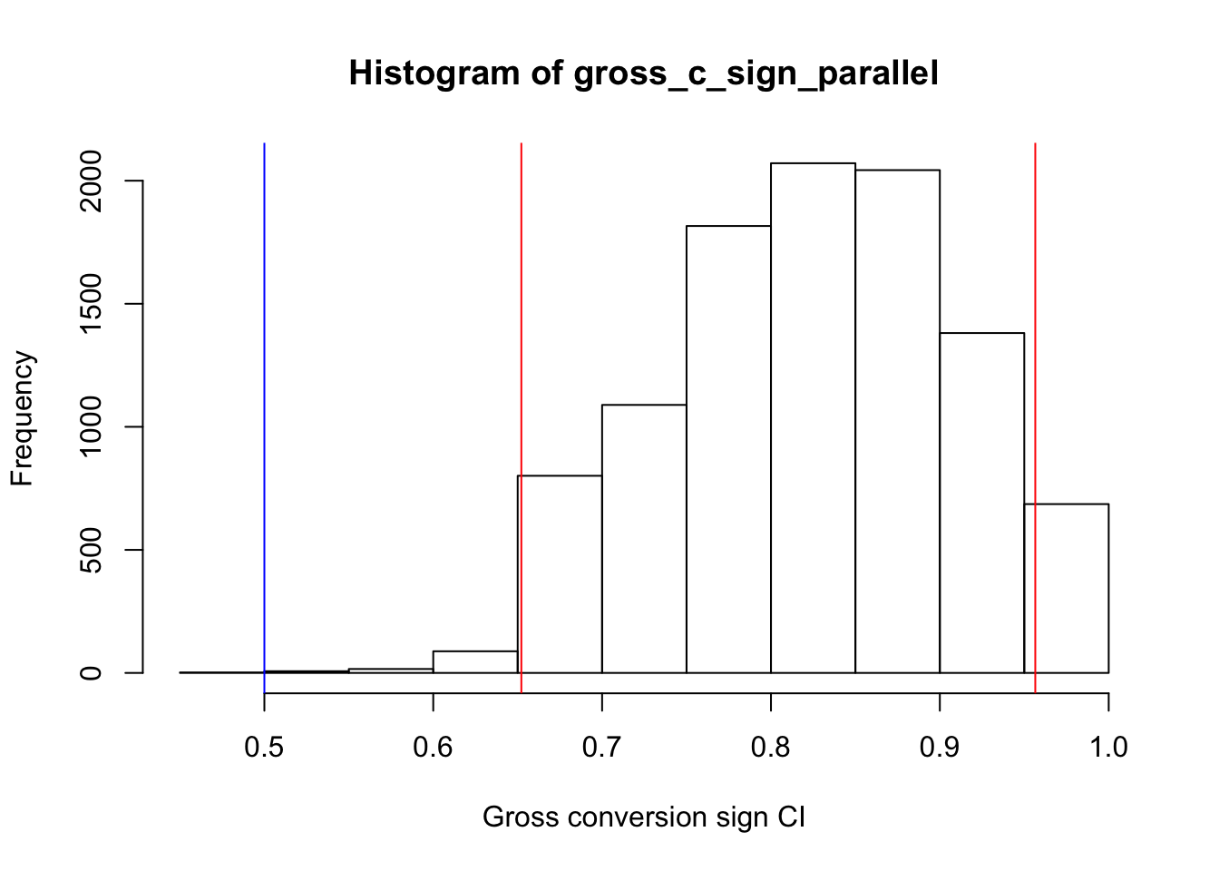
The gross conversion rate has a different story from the net conversion rate. The above graph shows that the signs of the gross conversion metric are not comming from a population with proportion = 0.5, so we reject this null hypothesis in favor of the alternate hypothesis.
The proportion of the negative signs in the gross conversion data is significantly higher than 0.5, and this assures us further that the gross conversion rate of the experiment group is significantly lower than the control group.
8. Recommendation Link to heading
This experiment aimed to assess whether filtering students based on their study time commitment would enhance the overall student experience and coaches’ ability to support those likely to complete the course, without significantly impacting the number of students who continue beyond the free trial. The results showed a statistically and practically significant decrease in Gross Conversion, but no notable differences in Net Conversion. This means there was a decrease in enrollment without a corresponding increase in students staying for the required 14 days to trigger payment. Based on these findings, it is recommended not to proceed with the launch and instead explore other experimental approaches.